Assumptions
In Knot Physics, spacetime is a branched 4-dimensional manifold embedded in a 6-dimensional Minkowski space. The spacetime manifold has constraints that relate its branching and its geometry. These assumptions fully specify Knot Physics with zero free parameters.
Spacetime is embedded in a larger space.
In Knot Physics, spacetime is a 4-dimensional manifold embedded in a 6-dimensional Minkowski space.
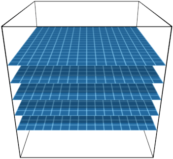
The spacetime manifold is branched.
The spacetime manifold is a branched manifold. Those branches can split and recombine.
There is a branch weight \(w\) that is conserved when the spacetime manifold branches.
We assume that there is a branch weight \(w\) that is defined at every point on the spacetime manifold and that branch weight is conserved when branches split and recombine. We constrain branch weight such that \(w \ge 1\) everywhere, which implies that a branch with branch weight \(w\) can split into at most \(w\) branches. For this reason, the spacetime manifold can split into only a finite number of branches.
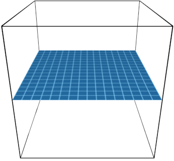
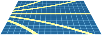
Branch weight is conserved when the spacetime manifold is stretched.
We assume that branch weight is conserved when the manifold stretches. Because \(w \ge 1,\) this constrains the spacetime manifold such that it can stretch by only a finite amount.
Branch weight conservation implies that branching and stretching are related.
Branch weight is conserved by both branching and stretching. The two constraints together imply a relationship between branching and stretching: As the manifold stretches, the branch weight decreases, and decreased branch weight allows fewer branches.
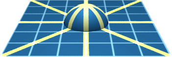
To describe stretching on a 4-dimensional manifold, we use curvature.
The spacetime manifold is a 4-dimensional manifold embedded in a 6-dimensional Minkowski space. The description of branch weight must be suitable for a manifold of these dimensions. In particular, the notion of “stretching” must include curvature. Increasing the scalar curvature of a manifold increases its volume. We construct our constraints on branch weight such that the branch weight is conserved even when the stretching is a consequence of curvature.
The following mathematical assumptions are the basis for all of Knot Physics.
The previous concepts can be incorporated into precise mathematical definitions, as follows.
The spacetime manifold is embedded in a larger space. The components of that embedding are:
- A 6-dimensional Minkowski space \( \Omega\)
- A 4-dimensional branched spacetime manifold \(M ,\) which is embedded in \(\Omega\)
We will use three metrics to describe the Minkowski space and the spacetime manifold:
- On the Minkowski space \(\Omega,\) there is the Minkowski metric \(\eta_{\mu\nu} = diag(1,-1,-1,-1,-1,-1).\)
- On the spacetime manifold \(M,\) there is the metric \(\bar{\eta}_{\mu\nu}\) which is the metric induced on \(M\) by its embedding in \(\Omega.\)
- There is also a metric \(h_{\mu\nu}\) on \(M\) which constrains the geometry and branching of \(M.\)
We want the metric \(h_{\mu\nu}\) to regulate the relationship between curvature and branch weight. We define the branch weight \(w\) to be the volume element of the metric \(h_{\mu\nu},\) which is to say \(w=(-\det (h))^{1/2}.\) We then require that the metric \(h_{\mu\nu}\) is Ricci flat. We write this constraint as \(\hat{R}^{\mu\nu} = 0.\) This constraint implies that the branch weight is conserved in a way similar to the stretching examples shown above. We include the constraint that the branch weight must be greater than or equal to 1 everywhere. We also require that branch weight is conserved when branches split and recombine.
This gives us our constraints on the manifold:
- The metric \(h_{\mu\nu}\) is Ricci flat, which we write \(\hat{R}^{\mu\nu}=0.\)
- The branch weight \(w = (-\det (h))^{1/2}\) must be \(w\ge1\) everywhere.
- The branch weight \(w\) is conserved when branches split and recombine.
In Knot Physics, all physical phenomena—including particles, quantum mechanics, and all forces—result from these assumptions.
To learn more, see [4]. These same assumptions can be stated in different ways, and they are presented differently in the papers. The mathematical content of the assumptions is the same.
Fermions
The constraints on the spacetime manifold allow it to pass through a singular state that produces a pair of topological defects, which we often refer to as knots. An elementary fermion consists of one knot on every branch of spacetime.
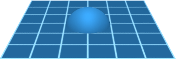
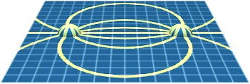
The manifold can pass through a singular state to produce a pair of fermions.
The spacetime manifold can create a pair of topological defects by passing through a singular intermediate state, which is analogous to pinching the manifold. This intermediate state is consistent with the constraints on the manifold. In particular, this pinching of the manifold is consistent with the constraint that the metric \(h_{\mu\nu}\) is Ricci flat. Annihilation is also possible through the same mechanism. The topological defects have homeomorphism class \(\mathbb{R}^3\#(S^1 \times P^2).\) These topological defects are the fermions of Knot Physics, and we often refer to them as "knots." The creation and annihilation of pairs of knots corresponds to the creation and annihilation of particle-antiparticle pairs.
Fermion generations correspond to different embeddings of knots.
The homeomorphism class \(\mathbb{R}^3\#(S^1\times P^2)\) can have multiple distinct embeddings. The different embeddings correspond to the generations of elementary fermions.
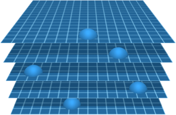
Spacetime is branched, and one fermion has one knot on every branch.
In Knot Physics, spacetime is a branched manifold. Previously, a fermion was simply defined as a knot in spacetime, but branched spacetime necessitates a more precise definition of a fermion: One fermion has one knot on every branch of spacetime. (For more about how knots behave on branches, see Quantum Mechanics.)
Quantum Mechanics
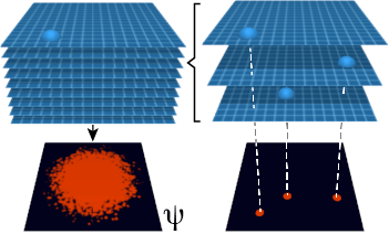
The branches of spacetime continually split and recombine. Recombination of the branches causes recombination of knots. Knot recombination produces quantum interference. Each branch can be considered a history in the sum-over-histories description of quantum mechanics.
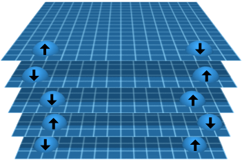
Branched spacetime allows quantum superposition.
A fermion consists of one knot on each branch of spacetime. Each knot can move around on its own branch, independently of the knots on other branches. Each branch is a state in a quantum superposition.
Knot geometry can be described using quantum amplitude.
Spacetime is a 4-dimensional manifold that is embedded in a 6-dimensional Minkowski space. The Minkowski space has 2 more dimensions than the manifold. Knots on the spacetime manifold can rotate and change size in those 2 additional dimensions. The rotation and size of the knot can be described with an angle \(\theta\) and magnitude \(r,\) or with a complex number \( k=re^{i\theta}.\) That complex number \(k\) is called the knot amplitude. Multiplying the knot amplitude \(k\) by the branch weight \(w\) produces a complex number \(wk,\) which is the quantum amplitude for the knot. (For more on branch weight, see Assumptions.)
Recombination of branches causes quantum interference.
When branches recombine, their knots can recombine. Knot amplitudes recombine to the weighted average. For example, suppose two recombining branches have branch weights \(w_1\) and \(w_2\) and knots that have knot amplitudes \(k_1\) and \(k_2.\) After recombination, the new knot has a knot amplitude \(k_3,\) which is the weighted average of the recombining knot amplitudes:
\(k_3 = \frac{w_1 k_1+w_2 k_2}{w_1+w_2}.\)
Because branch weight is conserved, the combined branch weight is
\(w_3 = w_1+w_2.\)
This implies that the quantum amplitudes of the knots are additive at recombination:
\(w_3 k_3=w_1 k_1+w_2 k_2.\)
This addition of quantum amplitudes is quantum interference.
The quantum wave function is the sum of the quantum amplitudes.
Spacetime consists of a large, but finite, number of branches. A fermion consists of a knot on each branch, and each knot has a quantum amplitude. The sum of the quantum amplitudes of the knots on all branches is the quantum wave function for the fermion.
The quantum amplitudes can be modeled with a path integral.
A path integral can be used to describe the diffusion and recombination of knots. The path integral is a continuous approximation of the discrete and finite system of branches and knots. Each branch can be considered a history in the sum-over-histories description of quantum mechanics.
The Born rule, which relates quantum amplitude to measurement probability, follows from knot geometry.
The probability of an event is proportional to the measure of the phase space in which that event happens. There are more ways to make a big knot than there are ways to make a small knot, and for that reason, events that involve big knots are more likely. The Born rule follows from the relationship between the quantum amplitude of a knot and the measure of phase space corresponding to that knot geometry.
Quantum entanglement results from the structure of the branches.
Each branch of spacetime has one quantum state for each particle. In this way, each branch selects combinations of quantum states. Entanglement between particles results when the selected combinations include correlations between particle states.
Entropy
The spacetime manifold is under-constrained; therefore, it has degrees of freedom. Subject to its constraints, the spacetime manifold maximizes entropy. Entropy maximization results in all of the dynamics of the spacetime manifold, including quantum wave function collapse. Entropy maximization can also be used to derive a Lagrangian.
The spacetime manifold maximizes entropy.
The spacetime manifold is constrained, but it is under-constrained. The spacetime manifold has entropy in the random behavior of its recombining branches and also in the spontaneous production of virtual particles. The spacetime manifold maximizes this entropy, subject to its constraints.
Entropy maximization implies branch cohesion.
Entropy is maximized when branches recombine frequently. Branches recombine frequently when branches remain similar. For this reason, entropy maximization implies that branches will stay similar to each other. This tendency to remain similar is called branch cohesion.
Branch cohesion implies wave function collapse.
The entropy of branch recombination causes branches to stay similar to each other. Because the branches must stay similar, it is not possible to have a quantum superposition with quantum states that are significantly different from each other. This implies that a quantum system that is evolving towards a superposition of highly dissimilar states will spontaneously collapse to one state or the other. For this reason, the entropy of branch recombination causes spontaneous wave function collapse.
Entropy maximization can be described using a Lagrangian.
The geometry of spacetime, including the presence of knots, affects the entropy of the spacetime manifold. Let \(\mathcal{L}\) be the amount by which the entropy is impaired relative to flat space with no particles. Then we can find a total entropy impairment \(S\) of a region \(A\) by integrating \(\mathcal{L}\) over that region, which is to say
\(S = \int_A \mathcal{L}\, \mathrm{d}M,\)
where \(\mathrm{d}M\) is the volume element of the spacetime manifold \(M.\) In this case, maximizing entropy implies minimizing the entropy impairment \(S.\) This is the same method that we use in the Standard Model when we minimize the action \(S\) associated to a Lagrangian \(\mathcal{L}.\)
Gravity
Matter impairs the entropy of the spacetime manifold. Curvature also impairs the entropy of the spacetime manifold. The spacetime manifold maximizes its entropy subject to these two factors. The result is gravity.
Stretching impairs entropy.
As shown in Assumptions, stretching the spacetime manifold reduces the number of branches. A reduction in the number of branches reduces branch recombination. This implies that stretching reduces entropy. For this reason, entropy maximization pulls back against stretching.
Scalar curvature impairs entropy.
Increasing the scalar curvature of spacetime implies stretching the spacetime manifold, which impairs entropy. For scalar curvature \(R\) and branch weight \(w,\) the entropy impairment of scalar curvature is \(wR.\) The entropy impairment over a region \(A\) is
\(S = \int_A wR \,\mathrm{d}M.\)
Matter impairs entropy.
The presence of matter and energy reduces the entropy of the spacetime manifold. The amount by which matter and energy impair entropy is proportional to the Lagrangian of matter and energy \(\mathcal{L}_m.\) For branch weight \(w,\) the entropy impairment as a result of matter and energy is \(w\mathcal{L}_m.\) The entropy impairment over a region \(A\) of spacetime is
\(S = \int_A w\mathcal{L}_m\, \mathrm{d}M.\)
Matter and scalar curvature both impair entropy.
Combining the entropy impairment of matter and curvature we get
\(S = \int w(\mathcal{L}_m + R)\mathrm{d}M.\)
If branch weight is constant, then entropy maximization is equivalent to the Einstein-Hilbert action.
With constant branch weight \(w,\) minimizing the entropy impairment equation
\(S = \int w(\mathcal{L}_m + R)\mathrm{d}M\)
is equivalent to minimizing the Einstein-Hilbert action,
\(S = \int (\mathcal{L}_m +R)\mathrm{d}M.\)
Over short distances, entropy maximization produces the Einstein-Hilbert action.
Entropy maximization causes branch weight to diffuse to a uniform distribution over short distances. This implies that the action of Knot Physics matches the action of general relativity over short distances.
Over large distances, entropy maximization may explain astronomical effects attributed to dark matter.
Over large distances, \(w\) may not be constant. This variation of branch weight may explain astronomical effects that are attributed to dark matter.
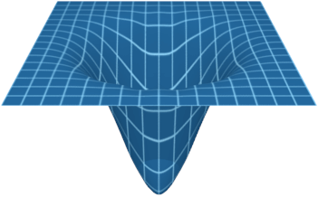
The Schwarzschild geometry can be embedded in a 6-dimensional Minkowski space.
In Knot Physics, the spacetime manifold is embedded in a 6-dimensional Minkowski space. In general relativity, the geometry of gravity for a single spherical mass is the Schwarzschild geometry. The Schwarzschild geometry can be embedded in a 6-dimensional Minkowski space. This result suggests that Knot Physics can reproduce the spacetime geometry for all gravitational geometries that have been observed.
Electromagnetism
The constraints on the spacetime manifold impair its entropy in a way that is independent of its geometry. That impairment of entropy can be characterized by a tensor that has the properties of the electromagnetic field tensor.
The electromagnetic field tensor \(F^{\mu\nu}\) is derived from the metric \(h_{\mu\nu}.\)
In Assumptions, we introduced the metric \(h_{\mu\nu},\) a rank two tensor that regulates branch weight. The spacetime manifold is constrained such that the metric \(h_{\mu\nu}\) is Ricci flat. This constraint affects the entropy of the spacetime manifold. We find an anti-symmetric tensor \(F^{\mu\nu},\) which is derived from the metric \(h_{\mu\nu},\) such that the entropy impairment is proportional to \(F^{\mu\nu}F_{\mu\nu}.\) We recall from Entropy that entropy impairment is the Lagrangian of Knot Physics; therefore, the Lagrangian of this field is proportional to \(F^{\mu\nu}F_{\mu\nu}.\) In this way, the tensor \(F^{\mu\nu}\) matches the electromagnetic field tensor of the Standard Model. The tensor \(F^{\mu\nu}\) is the electromagnetic field tensor of Knot Physics.
Knots can have charge.
Fermions are knots in spacetime, and those knots have a topology that can be a source of the electromagnetic field. Knots that are a source of the field are charged fermions.
To learn more, see [4].
Electroweak
Electroweak unification is a consequence of including knot geometry in the description of the electromagnetic field.
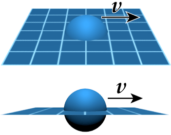
Knots have field energy, and the Lorentz transformations of that field energy depend on knot geometry.
The stress-energy tensor \(T^{\mu\nu}\) is defined at every point on the spacetime manifold, including points that are on a knot. If the knot is in motion, the velocity vector \(v\) of the knot will be parallel to flat spacetime. Because the knot geometry is not parallel to flat spacetime, the velocity vector of the knot motion may not be in the tangent space of the manifold on the knot. This causes the stress-energy tensor to Lorentz boost with rest mass. For this reason, field energy on a knot has rest mass.
On knots, the electromagnetic field has both energy and mass.
The electromagnetic field has energy; therefore, the electromagnetic field on a knot has mass.
Oscillations of the electromagnetic field on a knot propagate as Z bosons.
The Z boson is an oscillation of the electromagnetic field on a knot that leaves the charge unchanged. On a knot, the electromagnetic field has mass; therefore, the Z boson has mass.
Knots can transfer charge with a W boson.
Muon decay is an example of a W boson carrying charge on a knot. The charge of the muon transfers onto the electron via a W boson. The charge moves down the side of the muon knot, which is not parallel to flat spacetime; therefore, the W boson must have mass.
The Higgs boson is a transverse wave on spacetime.
When knots collide, their geometries respond elastically. In some cases, the collision can produce a transverse wave on the spacetime manifold. The wave is not parallel to flat spacetime; therefore, it has mass. The wave is topologically trivial, so it cannot be a fermion. It is the Higgs boson.
The gauge group of electroweak unification corresponds to rotations of the Minkowski 6-space.
In the Standard Model, electroweak unification describes symmetry breaking using the gauge group \(SU(2)\times U(1).\) This group can be understood as rotations of the Minkowski 6-space that leave components of the electroweak field invariant.
To learn more, see [4].
Strong Force
Knots can link to each other, and linked knots are quarks. Linked knots exhibit the characteristic behaviors of the strong force: asymptotic freedom, confinement, and gluons.

Quarks are linked knots.
An elementary fermion is a topological defect with homeomorphism class \( \mathbb{R}^3 \# (S^1 \times P^2),\) referred to here as a knot. Embeddings of these topological defects can link such that they cannot be separated from each other. Linked knots are quarks. For example, a proton consists of three linked knots.
Linking allows asymptotic freedom.
When the linked knots are closer to each other than the knot radius, they exert no force on each other. This is asymptotic freedom.
Linking causes confinement.
Because the knots are linked to each other, they cannot be separated. This is confinement.
Gluons are the force between linked knots.
When linked knots are pulled away from each other, they are pulled back by the other linked knots. This pulling force performs the same function as gluons do in the Standard Model.
QCD is a consequence of knot geometry.
The position of quarks can be described using vectors \(a,\) \(b,\) and \(c\) that are the displacement of each quark from the center of the particle.
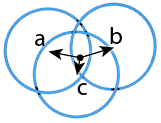
Knot Physics assumes that spacetime is embedded in a 6-dimensional Minkowski space, which has 5 spatial dimensions. Those displacement vectors are therefore 5 dimensional:
\(a = (a_1, a_2, a_3, a_4, a_5)\)
\(b = (b_1, b_2, b_3, b_4, b_5)\)
\(c = (c_1, c_2, c_3, c_4, c_5).\)
The center of the particle is the origin of coordinates, and this implies that the vectors sum to zero:
\(a+b+c=0.\)
The quarks cannot be separated from the particle, and this property can be represented by saying that these displacement vectors must have magnitude less than or equal to 1 in some units:
\(|a|\le 1\)
\(|b|\le 1\)
\(|c|\le 1.\)
This is equivalent to adding a sixth non-physical coordinate such that each vector has magnitude equal to 1:
\(|a'| = |(a_1, a_2, a_3, a_4, a_5, a_6)| = 1\)
\(|b'| = |(b_1, b_2, b_3, b_4, b_5, b_6)|=1\)
\(|c'| = |(c_1, c_2, c_3, c_4, c_5,c_6)|=1.\)
This is furthermore equivalent to converting each vector to a complex 3-vector:
\(|a''| = |(a_1+ a_2i, a_3+a_4i, a_5+a_6i)| = 1\)
\(|b''| = |(b_1+ b_2i, b_3+ b_4i, b_5+ b_6i)|=1\)
\(|c''| = |(c_1+ c_2i, c_3+ c_4i, c_5+c_6i)|=1.\)
Now each quark has a complex 3-vector of unit magnitude. The addition of the sixth coordinate implies that the vectors may not sum exactly to zero, but it will be a good estimate.
The linked knots can therefore be approximately described with complex 3-vectors of unit magnitude that sum to zero, which is the description of color charge. Furthermore, the quark displacements have no effect on the Lagrangian as long as the quarks are close enough to each other, which is guaranteed by the unit magnitude constraint. A gauge group can therefore be used. For complex 3-vectors, it suffices to use the gauge group \(SU(3).\) This reproduces the description of quantum chromodynamics.
To learn more, see [4].
More Results
The geometry of an electron knot allows a calculation of its spin angular momentum as a function of charge. Because the angular momentum is \(\hbar/2,\) the calculation allows a comparison of electron charge to Planck’s constant, which gives a derivation of the fine structure constant. The estimate is accurate to 0.1%. Calculation of additional Feynman diagrams may result in additional accuracy.
To learn more, see [5].
As discussed in Gravity, the branches of the spacetime manifold are constrained by branch weight, and the distribution of branch weight affects spacetime curvature. Branch weight distribution can explain curvature that is attributed to dark matter without the need for additional particles.
To learn more, see [8].
The spacetime manifold is embedded in a larger space, and expansion of the manifold corresponds to expansion as an embedding in the larger space. The velocity of that expansion contributes to the redshift from distant astrophysical sources. That additional contribution may explain some, or all, of the data that is currently used to infer the existence of dark energy.
To learn more, see [7].
References
Topics in Knot Physics
- Schrödinger’s Cat — Reconciling quantum and classical physics
- Visualizing Knots in Spacetime — A visual description of fermion topology
Videos
- Video: Quantum Mechanics — A 3-minute video on quantum mechanics
Papers
- Physics on a Branched Knotted Spacetime Manifold — A paper describing the core of the theory, which is necessary background for the rest of the papers
- Deriving the Fine Structure Constant
- Entanglement and Locality
- Dark Energy
- Dark Matter