The Pauli Exclusion Principle

The geometry of elementary fermions prevents identical fermions from occupying the same quantum state.

The Pauli Exclusion Principle

The geometry of elementary fermions prevents identical fermions from occupying the same quantum state.

In physics we observe that there is at most one fermion in a quantum state. For example, the 1s orbital of helium can have at most two electrons, and these electrons must have opposite spin and thus be in distinct quantum states. The observation that multiple fermions cannot occupy the same quantum state is called the Pauli exclusion principle.

In the Standard Model, the Pauli exclusion principle is the result of a special property of the quantum wave function of fermions. Specifically, the quantum wave function of fermions is antisymmetric: If identical fermions are swapped then the wave function of the fermions changes sign. If we have two identical fermions labeled \(A\) and \(B\), then we can write the wave function of the two fermions as \(ψ_{AB}\). Fermion exchange antisymmetry implies that swapping the labels \(A\) and \(B\) reverses the sign of the wave function. In other words, \(ψ_{BA}=–ψ_{AB}\). If the two fermions are assumed to occupy the same quantum state, then \(ψ_{AB}=ψ_{BA}\). These two equations together imply that \(ψ_{AB}=ψ_{BA}=0\). In other words, the probability of observing two identical fermions in the same quantum state is \(0\).

In Knot Physics, a geometric model of quantum mechanics and elementary particles results in properties that are similar to fermion exchange antisymmetry and produces the Pauli exclusion principle.

Quantum Mechanics on a Branched Spacetime Manifold

In this section, we provide a brief summary of quantum mechanics in Knot Physics for the purposes of describing the Pauli exclusion principle. (For more on quantum mechanics in Knot Physics, see Theory Summary: Quantum Mechanics.)

In Knot Physics, spacetime is a 4-dimensional manifold embedded in a 6-dimensional Minkowski space. The spacetime manifold is a branched manifold, and the branches can split and recombine.

Spacetime is a branched manifold. The branches can split and recombine.

We assume that there is a branch weight \(w\) that is defined at every point on the spacetime manifold and that branch weight is conserved when branches split and recombine. We constrain branch weight such that \(w≥1\) everywhere, which implies that a branch with branch weight \(w\) can split into at most \(w\) branches. For this reason, the spacetime manifold can split into only a finite number of branches.

Branch weight is additive at branch recombination.

Fermions—like electrons or quarks—are knots in the spacetime manifold.^[1] One fermion consists of one knot on every branch of spacetime. (In subsequent sections, we describe the topology of these fermion knots in detail.)

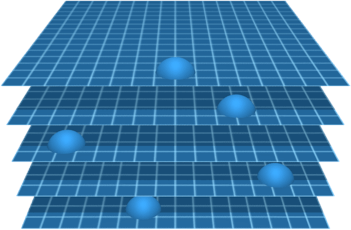
A fermion is one knot on each branch of the spacetime manifold — A single fermion—like an electron—consists of one knot on every branch of spacetime.

Each knot can move around on its own branch, independently of the knots on other branches. Each branch is a state in a quantum superposition.

Knot geometry can be described using quantum amplitude. Spacetime is embedded in a 6-dimensional Minkowski space, and knots on the spacetime manifold can rotate and change size in those two additional dimensions. Knot rotation and size can be described with an angle \(θ\) and magnitude \(\xi\), or with a complex number \( k=\xi e^{i\theta}.\) The complex number \(k\) is called the knot amplitude. Multiplying the knot amplitude \(k\) by the branch weight \(w\) produces a complex number \(wk\) , which is the quantum amplitude for the knot.

Two dimensions of the Minkowski space are perpendicular to the spacetime manifold. The knot can rotate in those two dimensions. This diagram does not have enough dimensions to portray that rotation, so the knot rotation is shown as if it were parallel to the spacetime manifold.

Recombination of branches causes quantum interference. When branches recombine, their knots can recombine. Knot amplitudes recombine to the weighted average. For example, suppose two recombining branches have branch weights \(w_1\) and \(w_2\) and knots that have knot amplitudes \(k_1\) and \(k_2.\) After recombination, the new knot has a knot amplitude \(k_3,\) which is the weighted average of the recombining knot amplitudes:

\(k_3 = \frac{w_1 k_1+w_2 k_2}{w_1+w_2}.\)

Because branch weight is conserved, the combined branch weight is

\(w_3 = w_1+w_2.\)

This implies that the quantum amplitudes of the knots are additive at recombination:

\(w_3 k_3=w_1 k_1+w_2 k_2.\)

This addition of quantum amplitudes is quantum interference.

One fermion has one knot on each branch of spacetime. Each knot can have its own quantum amplitude. When branches recombine, the knots on the branches also recombine. The quantum amplitude of the recombined knot is equal to the sum of the quantum amplitudes of the knots prior to recombination.

Spacetime consists of a large, but finite, number of branches. A fermion consists of a knot on each branch, and each knot has a quantum amplitude. The sum of the quantum amplitudes of the knots on all branches is the quantum wave function for the fermion.

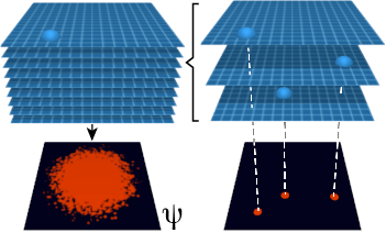
The quantum wave function is the sum of the quantum amplitudes on all branches — On the left, the sum of the quantum amplitudes of the knots on all branches produces a quantum wave function \(\psi.\) On the right, three branches are shown with their contributions to the quantum wave function.

The quantum amplitudes can be modeled with a path integral. A path integral can be used to describe the diffusion and recombination of knots. The path integral is a continuous approximation of the discrete and finite system of branches and knots. Each branch can be considered a history in the sum-over-histories description of quantum mechanics.

A Preview of the Pauli Exclusion Principle

In this section, we briefly outline how geometric interactions of fermion knots will result in the Pauli exclusion principle.

In subsequent sections, we will show that fermion knots affect each other geometrically as they pass each other and that this effect is equivalent to rotating the quantum amplitudes of those knots. This effect makes it impossible to have a quantum wave function with two fermions in the same quantum state. In other words, this geometric effect between fermion knots results in the Pauli exclusion principle.

To understand how the Pauli exclusion principle follows from this effect, we consider the hypothetical case that we have two fermions in the same quantum state. We consider two different interactions that both have the same start and end states. In case 1, two knots swap positions. In case 2, two knots approach each other and then return to their start positions.

Using the path integral formulation, the change in the quantum amplitudes of the knots depends on the action of the knots as they travel from their start positions to their end positions. The paths of the two cases are identical except for a small region of spacetime where the knots either pass or do not pass each other. We can choose paths that make the action of case 1 resemble the action of case 2 to arbitrary precision.^[2] If action were the only relevant variable for calculating the quantum amplitudes of the knots, then the changes in quantum amplitude of case 1 and case 2 would resemble each other to arbitrary precision.

In Knot Physics, an additional factor affects the quantum amplitudes of the knots: As the knots pass by each other, they interact geometrically, resulting in rotation of the quantum amplitudes of the knots. In case 1, the knots pass each other and therefore end with nonzero geometric interaction; in case 2, the knots do not pass each other and therefore end with zero geometric interaction. This difference in geometric interaction prevents the end-state quantum amplitudes of the two cases from converging, no matter how similar the actions of the two cases are.

We show two cases with identical fermions that occupy the same quantum state. In case 1 (left), two knots swap positions, and the quantum amplitudes of the knots are affected by their geometric interaction as they pass each other. In case 2 (right), two knots approach each other and then return to their start positions, and the end-state quantum amplitudes are unaffected by the knots’ interactions.

Because the quantum amplitudes do not converge to a unique value even for two approximately identical interactions, there can be no stable wave function for this system that has two fermions occupying the same quantum state.

Fermion Topology

The obstruction to two fermions occupying the same quantum state is a consequence of the geometric interaction between fermion knots as they pass by each other. To understand this effect, we first establish the topology of fermions.

A 2-dimensional Version of a Fermion Knot

As introduced previously, a fermion consists of one knot on each branch of spacetime. We can describe the topology of fermion knots using a process known as topological surgery, where we take familiar manifolds and then cut and glue them.^[3] We first use topological surgery to create the 2-dimensional version of a fermion knot, and we then extend the concept to 3 dimensions.

We begin with \( \mathbb{R}^2 ,\) which is a 2-dimensional plane. Then we perform a surgical operation by removing a disk \( D^2 \) from the plane. The result of that surgery is called \( \mathbb{R}^2 - D^2 .\) By removing the disk \( D^2\), we have created a boundary circle. The next step is to take every point on the boundary and attach it to the point that is diametrically opposite to it. It may seem like this would just close the hole that we created by removing the disk, but it actually creates something entirely new: the topological defect \( \mathbb{R}^2 \# P^2\), which we call a knot. The knot \( \mathbb{R}^2 \# P^2 \) is the 2-dimensional version of a fermion knot.

A disk \( D^2 \) has been removed from the plane \( \mathbb{R}^2 \), resulting in \( \mathbb{R}^2 - D^2 .\) The orange circle is the boundary where the disk has been removed. Then, every point on the boundary of the removed disk is attached to the point opposite to it, creating \( \mathbb{R}^2 \# P^2 .\) To fully show the geometry, we would need to portray 4 dimensions, which of course we cannot do. So in this animation, we show a 3-dimensional projection.

After this surgery, the manifold no longer fits in 2 dimensions. \( \mathbb{R}^2 \# P^2 \) must be embedded in a space with at least 4 dimensions, otherwise the manifold would intersect itself.

A Fermion Knot

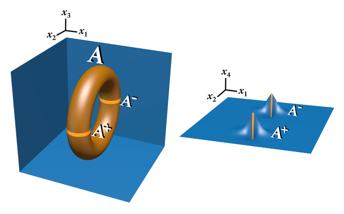
We now create the actual topology of fermion knots by extending the topological surgery operation to 3 dimensions. We begin with \( \mathbb{R}^3\), a 3-dimensional space. Then we perform a surgical operation by removing a solid torus \( S^1 \times D^2 \) from \( \mathbb{R}^3\) to create a boundary torus. The result is \( \mathbb{R}^3 - (S^1 \times D^2) .\)

We will refer to circles around the minor radius of the torus as boundary circles. Previously, we used the boundary circle of \( \mathbb{R}^2 - D^2 \) to make \( \mathbb{R}^2 \# P^2 \). Now, we perform that same surgery on the circles of the boundary torus: We attach each point on each circle to the point that is diametrically opposite to it. The result of that surgery is \( \mathbb{R}^3 \# (S^1 \times P^2) \).

By performing this topological surgery in 3 dimensions, we have created the topology of a fermion knot: \( \mathbb{R}^3 \# (S^1 \times P^2) \).^[4] After this surgery, the manifold must be embedded in a space with at least 5 dimensions; anything less than that would cause the manifold to intersect itself.

We remove a solid torus \( S^1 \times D^2 \) from \( \mathbb{R}^3\), resulting in \( \mathbb{R}^3 - (S^1 \times D^2) \) (left). Note that the orange torus is “hollow”: It is the boundary of the removed solid torus \( S^1 \times D^2 \). For each circle on the boundary torus (such as the circle highlighted in bright orange), every point is attached to the point opposite to it, creating \( \mathbb{R}^3 \# (S^1 \times P^2) \).

Because the surgery occurs in 5 dimensions, \((x_1,x_2,x_3,x_4,x_5)\), we hide and show different dimensions to see various features of the surgery.

On the left, we show the dimensions \((x_1,x_2,x_3)\). We see the boundary torus of \( \mathbb{R}^3 - (S^1 \times D^2) \) contracting as we attach each point on each circle of the torus to the point that is diametrically opposite to it.

On the right, instead of showing dimension \(x_3\), we show dimension \(x_4\). We see a slice of \( \mathbb{R}^3 - (S^1 \times D^2) ,\) a plane with a disk removed. Each point on the boundary circle attaches to the point that is diametrically opposite to it, creating the topological defect \( \mathbb{R}^2 \# P^2 \). This occurs for every boundary circle on the boundary torus.

Geometric Interaction between 2-dimensional Fermion Knots

In Knot Physics, translating fermion knots past each other affects their quantum amplitudes, thereby producing the Pauli exclusion principle. This change in quantum amplitude follows from the geometry of the 2-dimensional version of a fermion knot. In this section, we consider how translating 2-dimensional fermion knots around each other affects their quantum amplitudes.

Embeddings of the 2-dimensional Fermion Knot

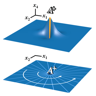
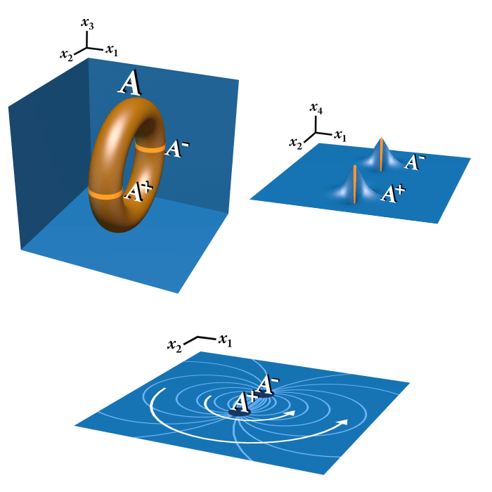
The fermion knot \( \mathbb{R}^3 \# (S^1 \times P^2) \) is a 3-dimensional manifold in a 5-dimensional space. The coordinates of the 5-dimensional space can be written \((x_1,x_2,x_3,x_4,x_5)\). Taking a 2-dimensional slice of the 3-dimensional fermion produces the topology \( \mathbb{R}^2 \# P^2 \), which is a 2-dimensional manifold embedded in a 4-dimensional space. To describe that space, we take a 4-dimensional slice through the 5-dimensional space by setting \(x_3=0\) to get coordinates \((x_1,x_2,0,x_4,x_5)\). The topology \( \mathbb{R}^2 \# P^2 \) is more conveniently understood using two polar coordinates, in which case we write the coordinates of this slice as \((r, σ, 0, x_4, x_5)\). The 2-dimensional topology \( \mathbb{R}^2 \# P^2 \) can then be understood as the following embedding in 4 dimensions, which we refer to as \(A^+\):

\(A^+=(r, σ, 0, \frac{1}{r+1}\cos(2σ), \frac{1}{r+1}\sin(2σ)\)).

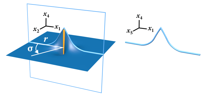
2-dimensional fermion knot with polar coordinates — On the left, we show the geometry of \( \mathbb{R}^2 \# P^2 \) as a slice through \(x_1x_2x_4\) with embedding \((r, σ, 0, \frac{1}{r+1}\cos(2σ), \frac{1}{r+1}\sin(2σ))\). On the right, we show the slice \(x_1x_4x_5\) at \(σ=0\) and \(σ=π\), which is \( (r, 0, 0, \frac{1}{r+1},0) \) and \( (r, π, 0, \frac{1}{r+1},0) \).

We see that this embedding performs the surgery that we associate with \( \mathbb{R}^2 \# P^2 \) by connecting a point at angle \(σ\) to the diametrically opposite point at \(σ+π\), because \(\sin(2(σ+π))=\sin(2σ)\) and \(\cos(2(σ+π))=\cos(2σ)\). The displacement into \(x_4x_5\) has magnitude \(\frac{1}{r+1}\), which is equal to \(1\) at \(r=0\) and diminishes to \(0\) at infinite distance.

The mirror image of this geometry, which we refer to as \(A^−\), reverses the orientation of the manifold by replacing \(σ\) with \(-σ\) in the \(x_4x_5\) coordinates:

\(A^-=(r, σ, 0, \frac{1}{r+1}\cos(-2σ), \frac{1}{r+1}\sin(-2σ)\)).

For both embeddings \(A^+\) and \(A^-\), rotation in the \(x_1x_2\) components is equivalent to rotation in the \(x_4x_5\) components. However, the differing geometries have two distinct symmetries such that the rotations in \(x_1x_2\) is equivalent to rotations in opposite directions in \(x_4x_5\).

These diagrams show the two embeddings of \( \mathbb{R}^2 \# P^2 \) (top and bottom) rotating in \(x_1x_2\). The light blue line indicates the slice \(x_2=0\). While the rotations of the two embeddings are identical in \(x_1x_2x_4\) (left), the two embeddings rotate in opposite directions in \(x_4x_5\) (right). Including the time parameter, these embeddings are \((r, σ, 0, \frac{1}{r+1}\cos(2(σ+t)), \frac{1}{r+1}\sin(2(σ+t)))\)(top) and \((r, σ, 0, \frac{1}{r+1}\cos(-2(σ+t)), \frac{1}{r+1}\sin(-2(σ+t)))\)(bottom).

The embeddings can scale by \(\xi\) and rotate by \(\theta\) in \(x_4x_5\). For example, scaling and rotating \(A^+\) produces \(A^+(\xi,\theta)\):

\(A^+(\xi,\theta)=(r, σ, 0, \frac{\xi}{r+1}\cos(2σ+\theta), \frac{\xi}{r+1}\sin(2σ+\theta)\)).

This embedding is a 2-dimensional fermion knot with knot amplitude \(k=\xi e^{i \theta}\). A magnitude \( \xi =1 \) and angle \( \theta =180°\), for example, would produce the embedding

\(A^+(1,180°)=(r, σ, 0, -\frac{1}{r+1}\cos(2σ), -\frac{1}{r+1}\sin(2σ)\)).

which rotates \(A^+\) by \(180°\) in \(x_4x_5\). This is equivalent to multiplying the knot amplitude of \(A^+\) by \(–1\).

Previously, we defined the quantum amplitude of the knot to be \(wk\) , where \(w\) is branch weight. In the following discussion, we assume that 2-dimensional fermion knots all have branch weight \(w=1\) so that we can conveniently refer to the knot amplitude as the quantum amplitude. As such, a \(180°\) rotation of \(A^+\) in \(x_4x_5\) is equivalent to multiplying the quantum amplitude of the 2-dimensional fermion knot by \(–1\).

Translating a Coordinate Frame around the 2-dimensional Fermion Knot

To understand the effect of translating 2-dimensional fermion knots past each other, we first establish the effect of translating a coordinate frame around a 2-dimensional fermion knot.

We note that there are two different methods of translating a coordinate frame in the \(x_1x_2\) plane. By one method, the coordinate frame has a vector that follows the tangent vector of its path of translation. By another method, the coordinate frame negates the rotation that results from its translation in \(x_1x_2\). This second method allows us to translate the coordinate frame in a way that does not depend on the shape of the path as a projection into \(x_1x_2\). We use this second method to describe translation around fermion knots because it represents the way that a fermion knot travels along a path without changing its spin angular momentum.

These diagrams depict two different types of translations of a coordinate frame on a flat \(x_1x_2\) plane. The top diagram shows the coordinate frame translating such that one of its basis vectors follows the tangent vector of the path of its translation. The bottom diagram shows the coordinate frame translating such that its basis vectors negate the effect associated with the projection of its path onto the \(x_1x_2\) plane.

We will use symmetries of the manifold to discern what happens to a coordinate frame as it translates around a 2-dimensional fermion knot. Translating a coordinate frame around the knot is equivalent to rotating the knot in \(x_1x_2\), and rotating the knot in \(x_1x_2\) is equivalent to rotating the knot in \(x_4x_5\). This implies that translation of the coordinate frame around the 2-dimensional fermion knot results in rotation of the coordinate frame in \(x_4x_5\). This relationship between translation and rotation of the coordinate frame is the key component of the geometric effect that occurs when fermion knots pass by each other.

A coordinate frame translates around a 2-dimensional fermion knot (top), and a coordinate frame holds still as a 2-dimensional fermion knot rotates (bottom).

The two distinct embeddings of the 2-dimensional fermion knot—\(A^+\) and \(A^-\)—produce two distinct rotations of the coordinate frame as it translates around the knot. For the embedding \(A^+\), translation of the coordinate frame in the \(+σ\) direction results in a rotation of the coordinate frame in the \(+x_4x_5\) direction. For the embedding \(A^−\), translation of the coordinate frame in the \(+σ\) direction results in a rotation of the coordinate frame in the \(–x_4x_5\) direction. In both cases, the knot geometry associates a rotation of magnitude \(2Δσ\) in \(x_4x_5\) for every translation of \(Δσ\) in \(x_1x_2\). This implies that translation of the coordinate frame by \(Δσ\) around \(A^+\) results in an \(x_4x_5\) rotation of \(+2Δσ\), and translation of the coordinate frame by \(Δσ\) around \(A^−\) results in an \(x_4x_5\) rotation of \(-2Δσ\).

Translating 2-dimensional Fermion Knots around Each Other

We now translate a 2-dimensional fermion knot around another 2-dimensional fermion knot—which is equivalent to the two knots swapping places—and consider the effect on the quantum amplitudes of those knots.

As previously described, a 2-dimensional fermion knot can be one of two embeddings: either \(A^+\) or \(A^-\). A pair of 2-dimensional fermion knots can therefore be one of four possible combinations: \(A^+B^+\), \(A^+B^−\) , \(A^−B^+\), or \(A^−B^−\). Only two unique combinations require consideration: \(A^+B^−\) and \(A^+B^+\).

We first consider the \(A^+B^−\) configuration. Swapping \(A^+\) and \(B^−\) is equivalent to \(B^−\) translating on a half circle around \(A^+\) such that \(B^−\) travels an angle \(Δσ=180°\) around \(A^+\). Translating \(B^−\) around \(A^+\) causes \(B^−\) to rotate in \(x_4x_5\) relative to \(A^+\) by an amount \(2Δσ=360°\). Because of the symmetry of \(B^−\), this is equivalent to rotating \(B^−\) in \(x_1x_2\) by \(180°\).

A 2-dimensional fermion \(B^−\) translates around \(A^+\) (top). The geometry of \(A^+\) causes \(B^−\) to rotate in the \(+x_4x_5\) direction as it translates (bottom). Because of the symmetry of \(B^−\), the rotation of \(B^−\) in \(x_4x_5\) is equivalent to rotation in \(x_1x_2\). Note that the rotation of \(B^-\) in \(x_1x_2\) is caused only by this symmetry; it is not directly caused by the translation of \(B^−\) in the \(x_1x_2\) plane.

Equivalently, we could translate \(A^+\) on a half-circle around \(B^−\) such that \(A^+\) travels an angle \(Δσ=180°\) around \(B^−\), which would cause \(A^+\) to rotate in \(x_4x_5\) relative to the geometry of \(B^−\) by an angle of \(-2Δσ\)=–360°. Because of the symmetry of \(A^+\), this is equivalent to rotating \(A^+\) in \(x_1x_2\) by \(180°\).

A 2-dimensional fermion \(A^+\) translates around \(B^−\) (top). The geometry of \(B^−\) causes \(A^+\) to rotate in the \(–x_4x_5\) direction as it translates, which by symmetry is equivalent to rotation in \(x_1x_2\) (bottom).

Regardless of whether we consider \(A^+\) to be rotating in \(x_4x_5\) relative to \(B^−\) or \(B^−\) to be rotating in \(x_4x_5\) relative to \(A^+\), \(A^+\) and \(B^−\) rotate relative to each other in \(x_4x_5\) in opposite directions by a total amount \(360°\). Since \(A^+\) and \(B^−\) are mirror images of each other, their rotations in \(x_4x_5\) are symmetric—equal in magnitude and opposite in direction. This implies that \(B^−\) experiences a rotation of \(+180°\) in \(x_4x_5\), and \(A^+\) experiences a rotation of \(−180°\) in \(x_4x_5\).

The 2-dimensional fermion knots \(A^+\) and \(B^−\) swap places (top). The geometry of the knots causes them to rotate in opposite directions in \(x_4x_5\) as they translate (bottom).

In the case that \(A^+\) and \(B^+\) swap places, the previous reasoning would imply that translating \(B^+\) around \(A^+\) would advance \(B^+\) by \(360°\) in \(x_4x_5\) relative to \(A^+\). Likewise, this reasoning would imply that translating \(A^+\) around \(B^+\) would advance \(A^+\) by \(360°\) in \(x_4x_5\) relative to \(B^+\). However, it is not possible for both of the 2-dimensional fermion knots to advance in angle in the same direction relative to each other. Using the symmetry between \(A^+\) and \(B^+\), we see that neither knot rotates in \(x_4x_5\). The geometry of each knot “pushes” against the other in an equal and opposite way resulting in an \(x_4x_5\) rotation of \(0°\) for both \(A^+\) and \(B^+\).

\(A^+\) and \(B^+\) swap places. The geometry of the 2-dimensional fermion knots results in neither knot rotating in \(x_4x_5\) as it translates.

Geometric Interaction between Fermion Knots

We now describe the geometric interaction between fermion knots by using the geometric interaction between a pair of 2-dimensional fermion knots. We will see how swapping fermion knots affects their quantum amplitudes.

Fermion Handedness

To evaluate the effect of swapping fermion knots, we first establish the relationship between a knot’s embedding and its spin angular momentum.

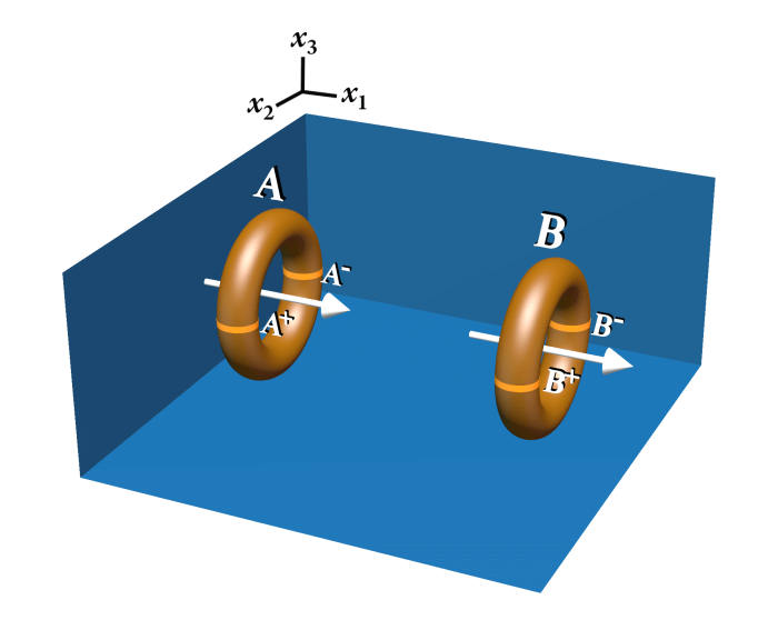
The fermion knot \( \mathbb{R}^3 \# (S^1 \times P^2) \) is a 3-dimensional manifold in a 5-dimensional space. We can consider a slice of the fermion knot by setting \(x_3\) constant. The resulting slice is a 2-dimensional manifold in a 4-dimensional space. The slice twice intersects the fermion knot, and at each intersection is the 2-dimensional version of a fermion knot, \( \mathbb{R}^2 \# P^2 \). We can label the fermion knot \(A\), in which case its slice has two 2-dimensional fermion knots with the embeddings \(A^+\) and \(A^-\).

The boundary torus associated with the topological surgery of the fermion knot and two 2-dimensional fermion knots — We show the boundary torus associated with the topological surgery of the fermion knot \( \mathbb{R}^3 \# (S^1 \times P^2) \), which we label \(A\) (left). If we take an \(x_1x_2x_4\) slice through the fermion knot \( \mathbb{R}^3 \# (S^1 \times P^2) \), there are two 2-dimensional fermion knots \( \mathbb{R}^2 \# P^2 \), which have the embeddings \(A^+\) and \(A^-\) (right).

The elementary fermion knot can rotate in its major and minor radii in a manner similar to a torus. The angular momentum associated with the rotation in the major radius of the fermion knot is the spin angular momentum of the elementary fermion. (For more information on spin angular momentum, see Physics on a Branched Knotted Spacetime Manifold ⇗)

The rotation of the fermion knot \(A\) in its major radius (as indicated by the white segment) corresponds to its spin angular momentum (which we denote with a white arrow) (left). The two 2-dimensional fermion knots \(A^+\) and \(A^-\) on the constant \(x_3\) slice do not rotate as a consequence of the spin angular momentum rotation (right).

The quantum amplitude of an elementary fermion advances in the manner prescribed by the Schrödinger equation. As discussed earlier, the quantum amplitude of the fermion corresponds to the quantum amplitude of its knots, and advance of the quantum amplitude of a fermion knot corresponds to the knot’s rotation in \(x_4x_5\).

As the fermion knot rotates in \(x_4x_5\), both 2-dimensional fermion knots on the constant \(x_3\) slice also rotate in the same direction in \(x_4x_5\) but in opposite directions from each other in \(x_1x_2\), which matches the previous discussion regarding rotations of the embeddings \(A^+\) and \(A^-\). In other words, the fermion knot’s rotation in \(x_4x_5\) corresponds to rotation in its minor radius.

Advance of the quantum amplitude of a fermion knot \(A\) corresponds to its rotation in \(x_4x_5\), which is equivalent to rotation of \(A\) in its minor radius (left). As \(A\) rotates in \(x_4x_5\), the two 2-dimensional fermion knots \(A^+\) and \(A^-\) on the constant \(x_3\) slice also rotate in \(x_4x_5\), which is equivalent to rotation of \(A^+\) and \(A^-\) in \(x_1x_2\) (right).

Based on observation, fermions have a property that breaks parity symmetry. In other words, for some physical experiments, it is possible to distinguish between a recording of the actual experiment or the mirror image of the actual experiment. This property of fermions is called fermion handedness.

In Knot Physics, fermion handedness results from a spontaneous symmetry breaking that relates fermion geometry to fermion rotation. In particular, fermion handedness couples the rotation of a fermion knot in its major radius to the rotation in its minor radius. (For more information about fermion handedness, see the papers Physics on a Branched Knotted Spacetime Manifold ⇗ and Knot Physics: Neutrino Helicity ⇗.)

As discussed previously, one of the 2-dimensional fermion knots in the constant \(x_3\) slice is the embedding \(A^+\) and the other is \(A^-\). Fermion handedness ensures that spin angular momentum is sufficient to determine which is \(A^+\) and which is \(A^-\). We will use this relationship between spin angular momentum and fermion embedding to determine how the quantum amplitude of fermion knots is affected when two fermion knots pass each other.

A constant \(x_3\) slice through a fermion knot has 2-dimensional fermion knots with embeddings \(A^+\) and \(A^-\) (right). Fermion handedness ensures that the direction of the spin angular momentum of a fermion knot determines which 2-dimensional fermion knot is \(A^+\) and which is \(A^-\).

Translating Fermion Knots around Each Other

Using the relationship between spin angular momentum and fermion embedding, we derive the change in quantum amplitude caused by fermion knots swapping places.

We first consider a pair of fermion knots \(A\) and \(B\) that have the same spin. A slice of constant \(x_3\) that passes through \(A\) and \(B\) contains four 2-dimensional fermion knots: \(A^+\), \(A^-\), \(B^+\), and \(B^-\).

Two fermion knots that have the same spin — A slice of constant \(x_3\) through two fermion knots \(A\) and \(B\) contains four 2-dimensional fermion knots: \(A^+\), \(A^-\), \(B^+\), and \(B^-\).

Fermion handedness implies that there is a consistent relationship between spin and fermion embedding. That relationship prescribes that as the two fermion knots \(A\) and \(B\) pass by each other, either \(A^+\) passes by \(B^-\) or \(B^+\) passes by \(A^-\). The resulting geometric interaction causes \(x_4x_5\) rotation of these fermions in a manner similar to the 2-dimensional case: One of the fermion knots experiences a rotation in the \(+x_4x_5\) direction, and the other experiences a rotation in the \(–x_4x_5\) direction. The direction of rotation in \(x_4x_5\) is determined by which of the pairs of 2-dimensional fermion knots pass most closely by each other. We recall that a rotation in \(x_4x_5\) of the fermion knot is equivalent to a rotation of its quantum amplitude.

A pair of fermion knots swap places (top). As they do, they rotate in \(x_4x_5\), which is equivalent to rotation of their minor radii. Synchronized with the top animation, two pairs of 2-dimensional fermion knots also swap places (middle and bottom). When \(A\) passes \(B\) such that \(A^+\) passes by \(B^−\) (top), the corresponding depiction (middle) is shown as “active”; when \(A\) passes \(B\) such that \(A^−\) passes by \(B^+\) (top), the corresponding depiction (bottom) is shown as “active.” The “active” depiction serves to indicate which of the pairs of 2-dimensional fermion knots approach most closely as the two fermion knots pass each other. The 2-dimensional fermion knots rotate in \(x_4x_5\) as they pass each other, which is equivalent to their rotation in \(x_1x_2\). This rotation corresponds to the rotation of the minor radii of the fermion knots.

In the other case, two fermion knots \(A\) and \(B\) have opposite spin. When \(A\) passes \(B\), \(A^+\) passes \(B^+\), and \(A^-\) passes \(B^-\). As with 2-dimensional fermions, this results in no angle change in \(x_4x_5\) for either of the fermion knots. In other words, two fermion knots of opposite spin do not affect each other’s quantum amplitude.

A pair of fermion knots with opposite spin swap places. During this swap, \(A^+\) passes \(B^+\), and \(A^-\) passes \(B^-\). As such, swapping the fermion knots does not induce a change of their quantum amplitudes.

We therefore have two unique cases. In the first case, fermion knots of the same spin swap places, and their quantum amplitudes change as a consequence of their geometric interactions. In the second case, fermion knots of opposite spin pass by each other, and their quantum amplitudes are unaffected by their geometric interactions.

Distance between Fermion Knots Affects Rotation

We now consider how the physical distance between swapped fermion knots influences their change in quantum amplitude.

The above presentation of geometric interaction between fermion knots is the naive extension of the arguments presented for the interaction of 2-dimensional fermion knots. We note, however, that the geometry around a fermion knot only locally resembles the geometry around a 2-dimensional fermion knot; at greater distances, this resemblance disappears. The geometry around a 2-dimensional fermion knot is distributed according to the angular coordinate of polar coordinates, whereas the geometry around a fermion knot is distributed according to the angular coordinate of toroidal coordinates. Taking this effect into account, a pair of fermion knots will affect each other less if they swap places by travelling along paths such that the two fermion knots remain far from each other relative to their size. For this reason, identical fermion knots that swap places while remaining far from each other will experience a lesser rotation in quantum amplitude.

2-dimensional ferimon knot and radial coordinates — The geometry associated with a 2-dimensional fermion knot (top) has a radial symmetry represented by polar coordinates (bottom). Translating a coordinate frame on a path around this 2-dimensional fermion knot causes a rotation of the coordinate frame in \(x_4x_5\) that is proportional to the number of radial lines that the path crosses. Regardless of whether the coordinate frame follows the inner path close to the knot or the outer path far from the knot, the number of radial lines crossed is the same.

Ferimon knot and toroidal coordinates — We consider a constant \(x_3\) slice (top right) that passes through a fermion knot \(A\) (top left) at \(A^+\) and \(A^-\). The slice has geometry that is distributed according to the angular coordinate of toroidal coordinates (bottom). Translating a coordinate frame on a path around this fermion knot causes a rotation of the coordinate frame in \(x_4x_5\) that is proportional to the number of coordinate lines that the path crosses. In this case, the inner path passes through more coordinate lines than the outer path. As such, translation of a coordinate frame along the inner path will result in greater rotation in \(x_4x_5\) than translation of the coordinate frame along the outer path.

The Pauli Exclusion Principle

Having established the relationship between translation of fermion knots and their quantum amplitudes, we now return to the hypothetical scenario in which two fermion knots share the same quantum state.

In Knot Physics, a fermion consists of one knot on every branch of spacetime. If there were two fermions in the same quantum state, then those fermions’ knots would often swap places while passing close to each other. When this happens, the geometric interaction between knots would affect their quantum amplitudes. As described previously, this geometric interaction prevents a stable wave function, thereby preventing the fermions from occupying the same quantum state. For this reason, the geometry of fermion knots results in the Pauli exclusion principle.

Notes

The mathematical theory of knots has a specific definition of the word “knot”: an embedding of an n-dimensional sphere \(S^n\) in an \(n+2\)-dimensional sphere \(S^{n+2}.\) In Knot Physics, we often use the term “knot” instead of “topological defect” for simplicity.
It may seem that the diameter of the knots prevents them from approaching each other any closer than the knot diameter. This is actually not an obstruction because fermion knots shrink as they approach each other. The spacetime manifold is constrained to be Ricci flat, and this flatness constraint requires that the knots get smaller as they get closer. This is also the reason that fermions appear pointlike in collisions. For more information, see Physics on a Branched Knotted Spacetime Manifold ⇗.
Topological surgery is a helpful way of understanding fermion topology. In reality, fermions are created and annihilated by an entirely different process. For more information on pair creation and annihilation, see Theory Summary: Fermions.
We have discussed the topology of fermions, specifically the homeomorphism class, which is \( \mathbb{R}^3 \# (S^1 \times P^2) \). This type of topological defect can have different embeddings and geometric properties. The variety of embeddings and geometric properties explains the variety of fermion types. For more information, see Physics on a Branched Knotted Spacetime Manifold ⇗.

Learn More

A natural transition from quantum to classical

Schrödinger’s Cat

At the center of physics is a conundrum that has persisted since the early days of quantum mechanics.

Superfluidity

In Knot Physics, superfluidity results from the properties of the branched spacetime manifold.

Theory Summary

An overview of the entire theory, from simple assumptions about the spacetime manifold through particles, quantum mechanics, and forces

Learn more

Theory Summary

An overview of the entire theory, from simple assumptions about the spacetime manifold through particles, quantum mechanics, and forces

Learn more