Theory Overview
Physics from the geometry of branched spacetime
Knot Physics explores whether matter, quantum mechanics, forces, and gravity can emerge from a branched, weighted spacetime.
The framework in brief
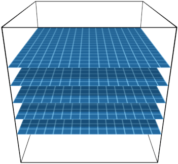
Spacetime is a branched four-dimensional manifold embedded in flat six-dimensional Minkowski space. Each branch is a complete candidate history with a positive weight. Matter consists of topological defects in the manifold. Quantum mechanics is the statistics of the branches, while forces arise from geometry and the entropy of branching and recombination.1
Knot Physics is an ongoing research program built around this developing theoretical framework. Knot Physics: A Complete Description of the Theory (opens in a new tab) explicitly distinguishes established results from modeling choices and unresolved work.2 Numbered footnotes link to the relevant passages in this volume (version 1.0).
Foundations
Axiom I: the branched weighted manifold
Each branch \(B_i\) carries a positive weight \(w_i=\rho_i^4\ge L>0\), where \(L\) is a universal floor. Weight is conserved when branches separate and recombine. A finite total weight can therefore support only finitely many branches. Choosing units with \(L=1\) gives the equivalent normalization \(w\ge1\). The theory presently treats the positive floor \(L\) as an axiom; neither its physical origin nor its numerical value has been derived.3
Axiom II: embedding, field map, and defects
Each branch is embedded by \(X:B\to\mathbb{R}^{5,1}\). It also carries an independent field map \(A:B\to\mathbb{R}^{5,1}\), with deviation \(\varepsilon=A-X\). The induced metric \(\bar\eta=X^*\eta\) measures lengths and proper time; the weight metric is \(h=\rho^2A^*\eta\). Defects have spatial-slice topology \(\mathbb{R}^3\#(S^1\times\mathbb{RP}^2)\), the normal 2-plane is spacelike, and branches do not self-intersect.4
The constraint and the dynamical postulate
The theory's field-equation-like constraint is \(\operatorname{Ric}[h]=0\) pointwise on every branch. It constrains the weight and field geometry; it does not say that the induced spacetime metric \(\bar\eta\) is flat. Subject to the axioms and constraint, the under-constrained branched manifold takes maximum-entropy configurations. The maximum-entropy postulate determines equilibrium and coarse-grained behavior, but the theory does not yet supply an irreversible microscopic law for each individual branching or recombination event.5
Matter as topological defects
A real fermion is a defect present on every branch. The defect construction supplies the spinorial double cover, the fermionic minus sign, and the exchange holonomy. Generations are identified with winding classes of the embedding; charge is a dynamical field-map fixed point rather than a topological label; linked defects are quarks. The theory classifies the observed particle slots, but it does not yet derive why the generation tower stops at three or compute the particle mass spectrum.6
For unlinked defects the charge fixed points are \(q\in\{0,\pm e\}\). Linked defects must be charged; third-integer quark charges are established at the level of linked-dressing consistency, while the complete derivation remains open. Confinement follows structurally from non-self-intersection: linked cores cannot be separated into a valid isolated-quark configuration.7
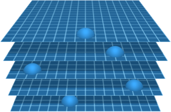
For an illustrated account of the defect construction, see Particle Topology.
Quantum mechanics from branch statistics
The wave function is the weighted branch sum \(\psi=\sum_i w_i a_i\), where the complex phase is the literal winding angle in the normal plane. At recombination the weighted-mean merge rule makes \(\psi\) additive. The rule is uniquely selected by symmetry, decomposability, and the quadratic reconfiguration cost, so linear superposition is derived within the framework.9
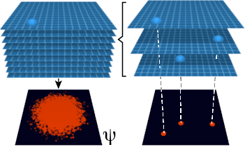
Defect cores follow piecewise-lightlike paths with reversals at the Compton rate. In the coarse-grained telegraph model, these reversals give diffusion constant \(D=\hbar/2m\), producing the Schrödinger coefficient; the topological winding of phase separately closes the usual Wallstrom circulation gap. The diffusion coefficient is established within this kinematic model; its full microscopic derivation still depends on uncomputed collision statistics and memory.11
The Born rule has two ingredients: pairwise branch-recombination counting supplies the quadratic structure, and the normal-plane state-space factor supplies the amplitude scaling. The pairing count is exact in the model, while a theorem-level derivation of one state-space scaling factor remains open. The framework therefore derives the quadratic pairing structure, but it does not yet provide the missing state-space theorem needed for a complete derivation of the Born measure.12
Collapse is a physical, threshold-driven instability. A macroscopic disagreement between branches carries an entropy cost proportional to its spacetime volume; above threshold, the superposed state becomes unstable and consolidates stochastically to one outcome. The mechanism and signatures are structured, but the escape rate, localization scale, and other numerical parameters wait on the uncomputed churn rate and memory kernel.13
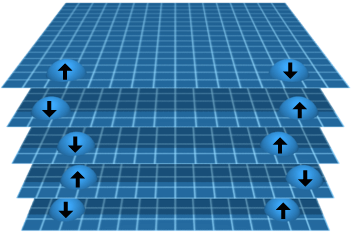
Pauli exclusion is topological and exact per branch: exchanging identical fermionic defects contributes a \(-1\) holonomy, so same-state occupancy requires \(a=-a=0\). The same-state channel cannot stabilize, while opposite-spin same-orbital states remain allowed. The mechanism predicts no finite-branch-number violation of exclusion.14
The impedance formulation
An impedance formulation packages phase and weight dynamics in \(P=i\hbar\,d\ln s\). Its imaginary/reactive sector describes phase rotation, stored structure, and unitary evolution; its real/resistive sector describes recombination, damping, decoherence, and decay. Mass and decay become the imaginary and real parts of one complex frequency. The formulation establishes the algebraic relation between reactive and dissipative sectors, but it does not yet determine most of the coefficients needed to predict absolute decay, decoherence, or collapse rates.15
Forces
Electromagnetism
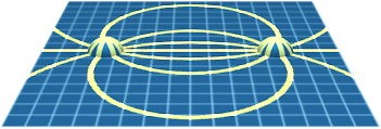
The electromagnetic field is the deviation \(\varepsilon=A-X\). The entropy expansion contains a weighted Maxwell term, reducing to Maxwell theory when \(w\) is constant. Normal-plane rotations give \(SO(2)\cong U(1)\). The charged-cusp calculation yields \(g=2\) at the order examined, and the null sector supplies a photon geometry. The framework has not yet derived the discrete photon spectrum or photon creation and annihilation directly from its branch and defect dynamics.16
Electroweak structure
The quaternionic ambient structure gives the \(U(2)\cong (SU(2)\times U(1))/\mathbb{Z}_2\) group structure at the group-theoretic and kinematic level. The photon is the split-preserving massless mode; the \(Z^0\) is a neutral codimensional shift; and \(W^\pm\) shifts carry both charged and codimensional components. Explicit dressed solutions for the massive bosons, their masses, and the weak mixing angle remain open. The Higgs field is the normal-plane coordinate and condensate. The free-energy argument fixes the potential's qualitative asymmetry, but its numerical self-couplings come only from a provisional calculation and have not been derived from the full dynamics.17
Strong sector
Quarks are linked defects. Confinement is the absence of an admissible separated configuration, not simply a pulling force. A seam between displaced linked cores supplies a model of the long-distance linear potential. The collision-transfer algebra closes on \(\mathfrak{su}(3)\), and removing the collective transfer mode leaves an octet exchange structure. These results reproduce parts of the kinematic color structure, but the theory has not yet constructed propagating gluon fields, derived the non-abelian beta function, fixed the dynamical weights, or calculated QCD scattering amplitudes.18
Gravity
The entropy expansion produces a weight-coupled Einstein–Hilbert term. Because the induced metric is a pullback rather than a free field, variation is over embeddings and yields the Regge–Teitelboim equation \((G^{\mu\nu}-\kappa T^{\mu\nu})K^I_{\mu\nu}=0\). Every Einstein solution satisfies this equation, but it is weaker than the Einstein equations. Connecting this effective equation to microscopic branch entropy requires a coarse-graining assumption that remains a postulate. Newton's constant and the general coarse-grained stress tensors of extended matter remain open computations.19
Quantitative results and honest boundaries
The flagship calculation gives the fine structure constant \(\alpha^{-1}_{\mathrm{calc}}\approx136.854\), compared with \(\alpha^{-1}_{\mathrm{exp}}\approx137.036\): a \(0.13\%\) discrepancy. The correction from virtual-particle screening has the required sign, but its magnitude in the stated scheme is uncomputed. The same constraint calculus gives the electron \(g=2\) at the order examined.20
The simplest generation-mass calculation fails decisively: it predicts \(1:\sqrt3:\sqrt5\), not the observed \(1:207:3477\). This rules out the simplest geometric mechanism and leaves the hierarchy to dynamics that have not yet been computed. Absolute masses, the generation hierarchy, CKM/PMNS structure, \(W/Z/H\) masses, the strong coupling, Newton's constant, photon quantization, and numerical collapse parameters remain open.21
Vacuum, dark matter, and cosmology
Knot Physics investigates whether the geometry and dynamics of branched spacetime can account for phenomena usually attributed to dark matter and dark energy. The present account combines a geometric mechanism with additional modeling assumptions; quantitative cosmological predictions remain under development.
Weight variations and dark matter
In the field-free regime, the weight metric \(h\) and the induced spacetime metric \(\bar{\eta}\) obey
Here \(w\) is the branch weight. The Ricci-flatness constraint applies to \(h\), while observers measure the geometry of \(\bar{\eta}\). In the weak-field treatment, spatial variations in weight provide a possible source of gravitational curvature without an additional matter particle. This is the proposed basis for the theory’s dark-matter account.
The halo picture adds assumptions about how weight is redistributed around galaxies. It suggests smooth central cores, a relationship between halo mass and a galaxy’s age and luminosity history, and an absence of isolated halos formed by the dark component’s own attraction. Quantitative halo profiles and the strength of these correlations remain to be calculated and compared with observations.22
Expansion and acceleration
The book explores inflation and late-time acceleration through an effective model of embedded spacetime that includes additional extrinsic-curvature, or “rigidity,” terms. These terms describe how the manifold bends in the surrounding space; their derivation from microscopic branch dynamics remains open.
A useful kinematic relation connects ambient time \(t\) to observers’ proper time \(\tau\):
Here \(v\) is the normal embedding velocity, \(c\) is the speed of light, and \(\mathcal{H}=a^{-1}da/dt\) and \(H=a^{-1}da/d\tau\) are expansion rates for the same scale factor \(a\). This relation explains how the two rates differ. Establishing accelerated expansion also requires equations for how the scale factor and lapse \(N\) evolve.
Within the effective model, the book reports an inflationary phase, an exit from inflation, and a late-time accelerating attractor. These results remain conditional on that model and its assumptions. The separate embedding redshift correction is insufficient by itself to account for the observed late-time acceleration. Deriving the rigidity coefficients, joining the two descriptions into one expansion history, and fitting that history to cosmological observations are explicit open problems.23
Empirical tests and discriminators
These proposals range from exact null predictions to parameter-dependent signatures. Where a required coefficient remains uncomputed, the item identifies an experimental target rather than a present numerical exclusion criterion.
- Mesoscopic quantum deviations: finite branch number predicts \(O(1/N)\) Born-rule deviations and event-localized energy non-conservation at collapse, while exchange holonomy predicts exactly zero stabilized Pauli violations. The rates remain uncomputed; any confirmed stabilized Pauli violation would directly falsify the holonomy mechanism.24
- Charge spectrum: the generation-blind fixed points are \(q\in\{0,\pm e\}\). A result \(\lvert q_\mu/q_e-1\rvert>10^{-9}\), or discovery of an elementary doubly charged lepton, would falsify the partition mechanism.25
- Higgs self-coupling: a provisional calculation of the entropic potential gives \(V'''b^*/V''=-1\), rather than \(+3\) for a symmetric quartic. A measured \((\lambda_3,\lambda_4)\) pair compatible only with the symmetric-quartic relation would falsify this mechanism; its absolute normalization remains uncomputed.26
- Dark-sector structure: the proposed weight-redistribution picture suggests cored halos, halo mass related to age and luminosity history, and no isolated halos formed through dark-sector self-attraction. These are qualitative targets; quantitative profiles and correlation strengths remain to be calculated.27
- Higher-order interference: a quartic state-space correction \(\epsilon\) would link half-period fringe contamination, \(c_2/c_1=\epsilon/[4(1+\epsilon)]\), to Sorkin interference, \(\kappa\approx4.5\epsilon\). Until \(\epsilon\) is calculated, this is a conditional signature rather than a standalone falsifier.28
- Primordial tensors: the effective embedded-inflation model describes a strongly suppressed tensor-to-scalar ratio, \(r\ll0.01\), with the suppression parametrized in the effective description. A confirmed primordial signal at \(r\gtrsim0.01\) would conflict with this proposed regime. The threshold tests those cosmological assumptions; it is not a model-independent prediction of the microscopic branched-manifold axioms.29
Explore the literature
Read the complete description of the theory alongside recent papers, published work, and topic-focused research documenting the development of Knot Physics.
View the literatureFootnotes
All notes refer to Knot Physics: A Complete Description of the Theory (opens in a new tab). Page numbers follow the book’s printed pagination.
- Ch. 1 · The theory in brief (opens in a new tab), pp. 2–3. Return to text
- Preface · What this document is and how to read it (opens in a new tab), pp. i–iii.The book’s status tags distinguish derivations within the framework from models, conjectures, and open problems. Return to text
- §2.2 · Axiom I: the branched weighted manifold (opens in a new tab), pp. 5–6; Appendix B · Map to the published axioms (opens in a new tab), p. 215. Return to text
- §2.3 · Axiom II: embedding and defects (opens in a new tab), pp. 6–8. Return to text
- §§2.4–2.5 · The constraint and Postulate III (opens in a new tab), pp. 8–10; §2.9 · What the foundations do not contain (opens in a new tab), p. 12. Return to text
- §§3.2–3.3 · Wrapping, spin, and the fermionic sign (opens in a new tab), pp. 14–16; §3.5 · Generations (opens in a new tab), pp. 17–18; §3.10 · The particle table (opens in a new tab), pp. 23–24.Topology permits both ordinary and spinorial fields; the constructed field selects the spinorial class. The identification of winding classes with generations is declared in the model. Return to text
- §§3.8–3.9 · Charge; quarks as linked defects (opens in a new tab), pp. 22–23. Return to text
- §3.7 · Pair creation and annihilation (opens in a new tab), pp. 18–19; §13.7 · The branched structure, explicitly: pair creation and amplitude splitting (opens in a new tab), pp. 88–89.The ribbon is a dimensional analogy. A complete constrained construction in three spatial dimensions plus time remains open. Return to text
- §§4.1–4.2 · The wave function and linear superposition (opens in a new tab), pp. 25–26; §24.3 · The merge theorem (opens in a new tab), pp. 134–135.The merge theorem uses the quadratic event-cost identification; weight-floor and core events delimit its scope. Return to text
- §4.8 · Entanglement and locality (opens in a new tab), pp. 32–34. Return to text
- §§4.3–4.4 · Phase, the Wallstrom point, and the Schrödinger equation (opens in a new tab), pp. 26–28; §25.4 · The lock, and its exposed coefficient (opens in a new tab), pp. 140–141.The diffusion coefficient depends on reversal statistics, not only on the mean Compton rate; the full collision and memory calculation remains open. Return to text
- §4.5 · The Born rule (opens in a new tab), pp. 28–30; §24.4 · The Born measure, and what it is not (opens in a new tab), p. 136. Return to text
- §4.7 · Collapse (opens in a new tab), pp. 31–32; §34.4 · The objective-collapse target space (opens in a new tab), pp. 183–184; §34.7 · The open front (opens in a new tab), p. 185. Return to text
- §4.9 · Exclusion (opens in a new tab), pp. 34–35.The exact null concerns stabilized same-state occupancy; transiently approachable configurations are distinguished from stabilized outcomes. Return to text
- §§5.1–5.3 · Two sectors, complex momentum, and complex frequency (opens in a new tab), pp. 36–38; §5.7 · The sector’s honest hinges (opens in a new tab), p. 40. Return to text
- §6.1 · Electromagnetism (opens in a new tab), pp. 41–42. Return to text
- §6.2 · The electroweak structure (opens in a new tab), pp. 42–45.The group relation is modulo the shared center. The boson descriptions are kinematic; the numerical Higgs self-couplings are provisional. Return to text
- §6.3 · The strong sector (opens in a new tab), pp. 45–48. Return to text
- §6.4 · Gravity (opens in a new tab), pp. 48–49; §§36.5–36.6 · The variation set and the genericity postulate (opens in a new tab), pp. 194–195.Embedding variation gives the Regge–Teitelboim equation. The step from microscopic entropy to the effective action relies on the stated genericity postulate. Return to text
- §7.1 · The fine structure constant: result and scope (opens in a new tab), pp. 52–53; §A.8 · The integral and the result (opens in a new tab), pp. 213–214; §6.1 · Electromagnetism: the magnetic moment (opens in a new tab), p. 42.The fine-structure calculation retains its stated model scope and two entropic selection principles. The screening correction’s sign is known; its magnitude is uncomputed. Return to text
- §§7.4–7.5 · Honest negatives and uncomputed quantities (opens in a new tab), pp. 55–56. Return to text
- §8.2 · Dark matter: weight without particles (opens in a new tab), p. 58; §10.5 · Cosmology, Problem C3 (opens in a new tab), pp. 67–68.The weak-field, field-free curvature mechanism is distinguished from the modeled transport layer; quantitative halo profiles and correlation strengths remain open. Return to text
- §§8.3–8.4 · Expansion and embedded cosmology (opens in a new tab), pp. 59–60; §10.5 · Cosmology, Problems C1–C2 (opens in a new tab), p. 67.The lapse relation is kinematic (with the speed of light restored explicitly here). The inflationary and late-time solutions depend on the effective action. Its rigidity coefficients have not been derived from branch entropy, and a unified expansion history and joint observational fit remain open. Return to text
- §§34.3–34.4 · The signature table and objective-collapse target space (opens in a new tab), pp. 182–184; §4.9 · Exclusion (opens in a new tab), pp. 34–35. Return to text
- §7.3 · The predictions register, items 2–3 (opens in a new tab), p. 54. Return to text
- §6.2 · The electroweak structure: the Higgs sector (opens in a new tab), p. 44; §7.3 · The predictions register, item 4 (opens in a new tab), p. 54.The self-coupling ratio is a provisional model-level result, not a fully derived numerical prediction. Return to text
- §8.2 · Dark matter: weight without particles (opens in a new tab), p. 58; §10.5 · Cosmology, Problem C3 (opens in a new tab), pp. 67–68. Return to text
- §7.3 · The predictions register, item 8 (opens in a new tab), p. 54. Return to text
- §8.4 · Embedded cosmology: the perturbation sector (opens in a new tab), p. 60.The book labels the result as derived within the effective action, with tensor suppression parametrized. The quoted threshold is conditional on that description; it is not a general numerical prediction of the microscopic axioms. Return to text